Scenic Fundamentals

This tutorial motivates and illustrates the main features of Scenic, focusing on aspects of the language that make it particularly well-suited for describing geometric scenarios. We begin by walking through Scenic’s core features from first principles, using simple toy examples displayed in Scenic’s built-in visualizer. We then consider discuss two case studies in depth: using Scenic to generate traffic scenes to test and train autonomous cars (as in [F22], [F19]), and testing a motion planning algorithm for a Mars rover able to climb over rocks. These examples show Scenic interfacing with actual simulators, and demonstrate how it can be applied to real problems.

We’ll focus here on the spatial aspects of scenarios; for adding temporal dynamics to a scenario, see our page on Dynamic Scenarios.

Objects, Geometry, and Specifiers

To start with, we’ll construct a very basic Scenic program:

ego = new Object

Running this program should cause a window to pop up, looking like this:

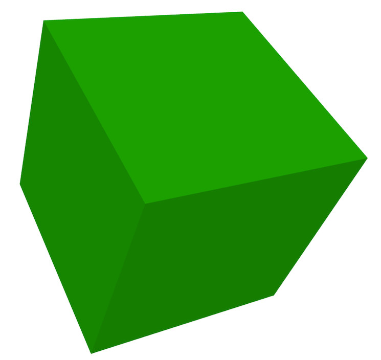
You can rotate and move the camera of the visualizer around using the mouse. The only Object currently present is the one we created using the new keyword (rendered as a green box). Since we assigned this object to the ego name, it has special significance to Scenic, as we’ll see later. For now it only has the effect of highlighting the object green in Scenic’s visualizer. Pressing w will render all objects as wireframes, which will allow you to see the coordinate axes in the center of the ego object (at the origin).

Since we didn’t provide any additional information to Scenic about this object, its properties like position, orientation, width, etc. were assigned default values from the object’s class: here, the built-in class Object, representing a physical object. So we end up with a generic cube at the origin. To define the properties of an object, Scenic provides a flexible system of specifiers based on the many ways one can describe the position and orientation of an object in natural language. We can see a few of these specifiers in action in the following slightly more complex program (see the Syntax Guide for a summary of all the specifiers, and the Specifiers Reference for detailed definitions):

ego = new Object with shape ConeShape(),
        with width 2,
        with length 2,
        with height 1.5,
        facing (-90 deg, 45 deg, 0)

chair = new Object at (4,0,2),
            with shape MeshShape.fromFile(localPath("meshes/chair.obj"),
                initial_rotation=(0,90 deg,0), dimensions=(1,1,1))

plane_shape = MeshShape.fromFile(path=localPath("meshes/plane.obj"))

plane = new Object left of chair by 1,
            with shape plane_shape,
            with width 2,
            with length 2,
            with height 1,
            facing directly toward ego

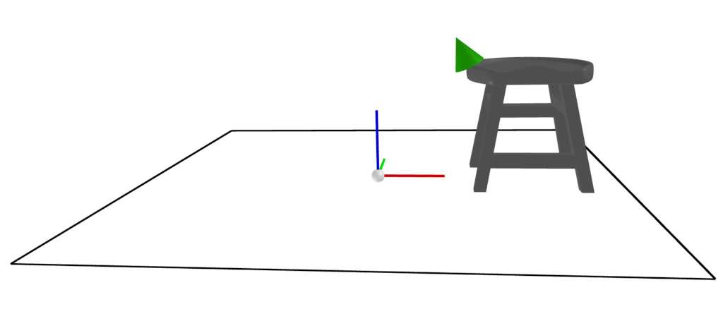
This should generate the following scene:

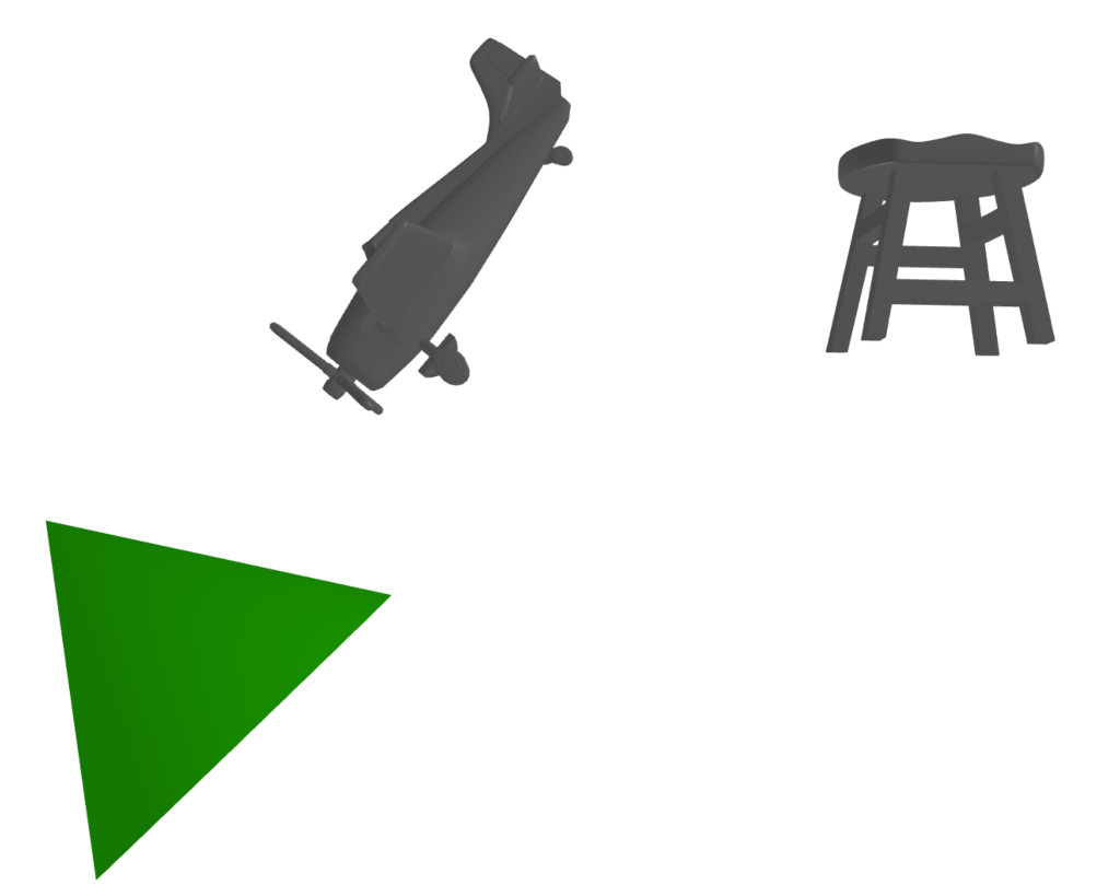
The first object we create, the ego, has a cone shape. Scenic provides several built-in shapes like this (see Shape for a list). We then set the object’s dimensions using the with specifier, which can set any property (even properties not built into Scenic, which you might access in your own code or which a particular simulator might understand). Finally, we set the object’s global orientation (its orientation property) using the facing specifier. The tuple after facing contains the Euler angles of the desired orientation (yaw, pitch, roll).

The second object we create is first placed at a specific point in space using the at specifier (setting the object’s position property). We then set its shape to one imported from a mesh file, using the MeshShape class, applying an initial rotation to tell Scenic which side of the chair is its front. We also set default dimensions of the shape, which the object will then automatically inherit. If we hadn’t set these default dimensions, Scenic would automatically infer the dimensions from the mesh file.

On line 11 we load a shape from a file, specifically to highlight that since Scenic is built on top of Python, we can write arbitrary Python expressions in Scenic (with some exceptions).

For our third and final object, we use the left of specifier to place it to the left of chair (the second object) by 1 unit. We set its shape and dimensions, similar to before, and then orient it to face directly toward the ego object using the facing directly toward specifier. This gives a first hint of the power of specifiers, with Scenic automatically working out how to compute the object’s orientation so that it faces the ego regardless of how we specified its position (in fact, we could move the left of specifier to be after the facing directly toward and the code would still work).

Scenic will automatically reject scenarios that don’t make physical sense, for instance when objects intersect each other [1]. For an example of this, try changing the code above to have a much larger ego object, to the point where it would intersect with the plane. While this isn’t too important in the scenarios we’ve seen so far, it becomes very useful when we start constructing random scenarios.

Randomness and Regions

So far all of our Scenic programs have defined concrete scenes, i.e. they uniquely define all the aspects of a scene, so every time we run the program we’ll get the same scene. This is because so far we haven’t introduced any randomness. Scenic is a probabilistic programming language, meaning a single Scenic program can in fact define a probability distribution over many possible scenes.

Let’s look at a simple Scenic program with some random elements:

ego = new Object with shape Uniform(BoxShape(), SpheroidShape(), ConeShape()),
                 with width Range(1,2),
                 with length Range(1,2),
                 with height Range(1,3),
                 facing (Range(0,360) deg, Range(0,360) deg, Range(0,360) deg)

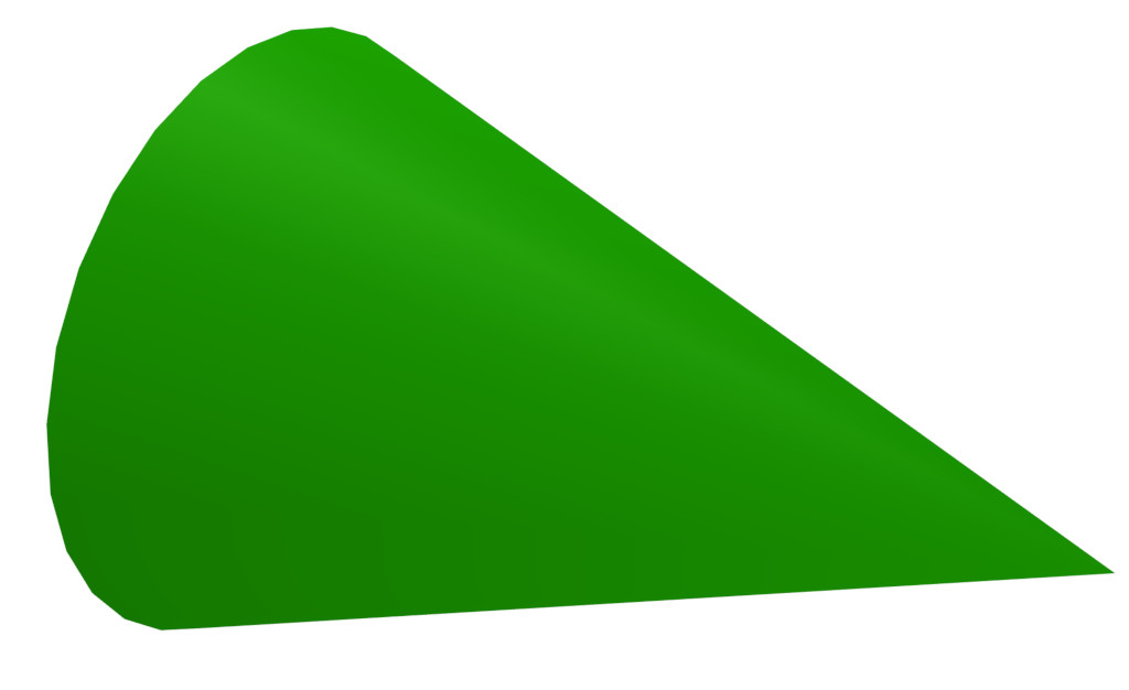
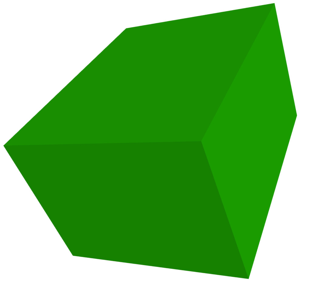
This will generate an object with a shape that is either a box, a spheroid, or a cone (each with equal probability). It will have a random width, length, and height within the ranges specified, and uniformly random rotation angles. Some examples:

Random values can be used almost everywhere in Scenic; the major exception is that control flow (e.g. if statements and for loops) cannot depend on random values. This restriction enables more efficient sampling (see [F19]) and can often be worked around: for example it is still possible to select random elements satisfying desired criteria from lists (see filter).

Another key construct in Scenic is a Region, which represents a set of points in space. Having defined a region of interest, for example a lane of a road, you can then sample points from it, check whether objects are contained in it, etc. You can also use a region to define the workspace, a designated region which all objects in the scenario must be contained in (useful, for example, if the simulated world has fixed obstacles that Scenic objects should not intersect). For example, the following code:

region = RectangularRegion((0,0,0), 0, 10, 10)
workspace = Workspace(region)

new Object in region, with shape SpheroidShape()
new Object in region, with shape SpheroidShape()
new Object in region, with shape SpheroidShape()

should generate a scene similar to this:

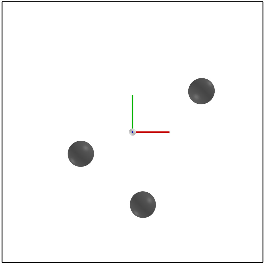
Note that in this scene the coordinate axes in the center are displayed due to the --axes flag, which can help clarify orientation.

We first create a 10-unit square RectangularRegion, and set it as the scenario’s workspace. RectangularRegion is a 2D region, meaning it does not have a volume and therefore can’t really contain objects. It is still a valid workspace, however, since for containment checks involving 2D regions, Scenic automatically uses the region’s footprint, which extends infinitely in the positive and negative Z directions. We then create 3 spherical objects and place them using the in specifier, which sets the position of an object (its center) to a uniformly-random point in the given region.

Similarly, we can use the on specifier to place the base of an object uniformly at random in a region, where the base is by default the center of the bottom side of its bounding box. The on specifier is also overloaded to work on objects, by default extracting the top surface of the object’s mesh and placing the object on that. This can lead to very compact syntax for randomly placing objects on others, as seen in the following example:

workspace = Workspace(RectangularRegion((0,0,0), 0, 4, 4))
floor = workspace

chair = new Object on floor,
            with shape MeshShape.fromFile(path=localPath("meshes/chair.obj"),
                dimensions=(1,1,1), initial_rotation=(0, 90 deg, 0))

ego = new Object on chair,
            with shape ConeShape(dimensions=(0.25,0.25,0.25))

which might generate something like this:

Orientations in Depth

Notice how in the last example the cone is oriented to be tangent with the curved surface of the chair, even though we never set an orientation with facing. To explain this behavior, we need to look deeper into Scenic’s orientation system. All objects have an orientation property, which is their orientation in global coordinates [2]. If you just want to set the orientation by giving explicit angles in global coordinates, you can use the facing specifier as we saw above. However, it’s often useful to specify the orientation of an object in terms of some other coordinate system, for instance that of another object. To support such use cases, Scenic does not allow directly setting the value of orientation using with: instead, its value is derived from the values of 4 other properties, parentOrientation, yaw, pitch, and roll. The parentOrientation property defines the parent orientation of the object, which is the orientation with respect to which the (intrinsic Euler) angles yaw, pitch, and roll are interpreted. Specifically, orientation is obtained as follows:

1. start from parentOrientation;

2. apply a yaw (a CCW rotation around the positive Z axis) of yaw;

3. apply a pitch (a CCW rotation around the resulting positive X axis) of pitch;

4. apply a roll (a CCW rotation around the resulting positive Y axis) of roll.

By default, parentOrientation is aligned with the global coordinate system, so that yaw for example is just the angle by which to rotate the object around the Z axis (this corresponds to the heading property in older versions of Scenic). But by setting parentOrientation to the orientation of another object, we can easily compose rotations together: “face the same way as the plane, but upside-down” could be implemented with parentOrientation plane.orientation, with roll 180 deg.

In fact it is often unnecessary to set parentOrientation yourself, since many of Scenic’s specifiers do so automatically when there is a natural choice of orientation to use. This includes all specifiers which position one object in terms of another: if we write new Object ahead of plane by 100, the ahead of specifier specifies position to be 100 meters ahead of the plane but also specifies parentOrientation to be plane.orientation. So by default the new object will be oriented the same way as the plane; to implement the “upside-down” part, we could simply write new Object ahead of plane by 100, with roll 180 deg. Importantly, the ahead of specifier here only specifies parentOrientation optionally, giving it a new default value: if you want a different value, you can override that default by explicitly writing with parentOrientation value. (We’ll return to how Scenic manages default values and “optional” specifications later.)

Another case where a specifier sets parentOrientation automatically is our cone-on-a-chair example above: in the code new Object on chair, the on specifier not only specifies position to be a random point on the top surface of the chair but also specifies parentOrientation to be an orientation tangent to the surface at that point. Thus the cone lies flat on the surface by default without our needing to specify its orientation; we could even add code like with roll 45 deg to rotate the cone while keeping it tangent with the surface.

In general, the on region specifier specifies parentOrientation whenever the region in question has a preferred orientation: a Vector Field (another primitive Scenic type) which defines an orientation at each point in the region. The class MeshSurfaceRegion, used to represent surfaces of an object, has a default preferred orientation which is tangent to the surface, allowing us to easily place objects on irregular surfaces as we’ve seen. Preferred orientations can also be convenient for modeling the nominal driving direction on roads, for example (we’ll return to this use case below).

Points, Oriented Points, and Classes

We’ve seen that Scenic has a built-in class Object for representing physical objects, and that individual objects are instantiated using the new keyword. Object is actually the bottom class in a hierarchy of built-in Scenic classes that support this syntax: its superclass is OrientedPoint, whose superclass in turn is Point. The base class Point provides the position property, while its subclass OrientedPoint adds orientation (plus parentOrientation, yaw, etc.). These two classes do not represent physical objects and aren’t included in scenes generated by Scenic, but they provide a convenient way to use specifier syntax to construct positions and orientations for later use without creating actual objects. A Point can be used anywhere where a vector is expected (e.g. at point), and an OrientedPoint can also be used anywhere where an orientation is expected. With both a position and an orientation, an OrientedPoint defines a local coordinate system, and so can be used with specifiers like ahead of to position objects:

spot = new OrientedPoint on curb
new Object left of spot by 0.25

Here, suppose curb is a region with a preferred orientation aligned with the plane of the road and along the curb; then the first line creates an OrientedPoint at a uniformly-random position on the curb, oriented along the curb. So the second line then creates an Object offset 0.25 meters into the road, regardless of which direction the road happens to run in the global coordinate system.

Scenic also allows users to define their own classes. In our earlier example placing spheres in a region, we explicitly wrote out the specifiers for each object we created even though they were all identical. Such repetition can often be avoided by using functions and loops, and by defining a class of object providing new default values for properties of interest. Our example could be equivalently written:

workspace = Workspace(RectangularRegion((0,0,0), 0, 10, 10))

class SphereObject:
    position: new Point in workspace
    shape: SpheroidShape()

for i in range(3):
    new SphereObject

Here we define the SphereObject class, providing new default values for the position and shape properties, overriding those inherited from Object (the default superclass if none is explicitly given). So for example the default position for a SphereObject is the expression new Point in workspace, which creates a Point that can be automatically interpreted as a position. This gives us a way to get the convenience of specifiers in class definitions. Note that this is a random expression, and it is evaluated independently each time a SphereObject is defined; so the loop creates 3 objects which will all have different positions (and as usual Scenic will ensure they do not overlap). We can still override the default value as needed: adding the line new SphereObject at (0,0,5) would create a SphereObject which still used the default value of shape but whose position is exactly (0,0,5).

In addition to the special syntax seen above for defining properties of a class and instantiating an instance of a class, Scenic classes support inheritance and methods in the same way as Python:

class Vehicle:
    pass
class Taxicab(Vehicle):
    magicNumber: 42

    def myMethod(self, x):
        return self.width + self.magicNumber + x

ego = new Taxicab with magicNumber 1729
y = ego.myMethod(3.14)

Models and Simulators

For the next part of this tutorial, we’ll move beyond the internal Scenic visualizer to an actual simulator. Specifically, we will consider examples from our case study using Scenic to generate traffic scenes in GTA V to test and train autonomous cars ([F19], [F22]).

To start, suppose we want scenes of one car viewed from another on the road. We can write this very concisely in Scenic:

from scenic.simulators.gta.model import Car
ego = new Car
new Car

Line 1 imports the GTA world model, a Scenic library defining everything specific to our GTA interface. This includes the definition of the class Car, as well as information about the road geometry that we’ll see later. We’ll suppress this import statement in subsequent examples.

Line 2 then creates a Car and assigns it to the special variable ego specifying the ego object, which we’ve seen before. This is the reference point for the scenario: our simulator interfaces typically use it as the viewpoint for rendering images, and many of Scenic’s geometric operators use ego by default when a position is left implicit [3].

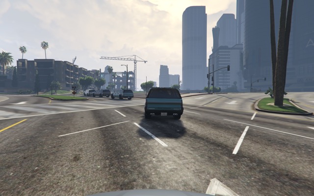
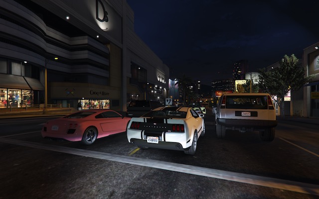
Finally, line 3 creates a second Car. Compiling this scenario with Scenic, sampling a scene from it, and importing the scene into GTA V yields an image like this:

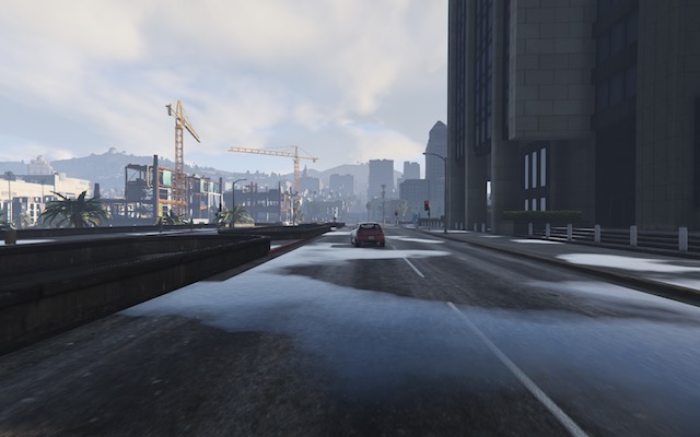
A scene sampled from the simple car scenario, rendered in GTA V.

Note that both the ego car (where the camera is located) and the second car are both located on the road and facing along it, despite the fact that the code above does not specify the position or any other properties of the two cars. This is because reasonable default values for these properties have already been defined in the Car definition (shown here slightly simplified):

class Car:
    position: new Point on road
    heading: roadDirection at self.position    # note: can only set `heading` in 2D mode
    width: self.model.width
    length: self.model.length
    model: CarModel.defaultModel()      # a distribution over several car models
    requireVisible: True    # so all cars appear in the rendered images

Here road is a region defined in the gta model to specify which points in the workspace are on a road. Similarly, roadDirection is a Vector Field specifying the nominal traffic direction at such points. The operator F at X simply gets the direction of the field F at point X, so line 3 sets a Car’s default heading to be the road direction at its position. The default position, in turn, is a new Point on road, which means a uniformly random point on the road. Thus, in our simple scenario above both cars will be placed on the road facing a reasonable direction, without our having to specify this explicitly.

One further point of interest in the code above is that the default value for heading depends on the value of position, and the default values of width and length depend on model. Scenic allows default value expressions to use the special syntax self.property to refer to the value of another property of the object being defined: Scenic tracks the resulting dependencies and evaluates the expressions in an appropriate order (or raises an error if there are any cyclic dependencies). This capability is also frequently used by specifiers, as we explain next.

Specifiers in Depth

Why Specifiers?

The syntax left of X and facing Y for specifying positions and orientations may seem unusual compared to typical constructors in object-oriented languages. There are two reasons why Scenic uses this kind of syntax: first, readability. The second is more subtle and based on the fact that in natural language there are many ways to specify positions and other properties, some of which interact with each other. Consider the following ways one might describe the location of a car:

1. “is at position X” (an absolute position)

2. “is just left of position X” (a position based on orientation)

3. “is 3 m West of the taxi” (a relative position)

4. “is 3 m left of the taxi” (a local coordinate system)

5. “is one lane left of the taxi” (another local coordinate system)

6. “appears to be 10 m behind the taxi” (relative to the line of sight)

7. “is 10 m along the road from the taxi” (following a potentially-curving vector field)

These are all fundamentally different from each other: for example, (4) and (5) differ if the taxi is not parallel to the lane.

Furthermore, these specifications combine other properties of the object in different ways: to place the object “just left of” a position, we must first know the object’s orientation; whereas if we wanted to face the object “towards” a location, we must instead know its position. There can be chains of such dependencies: for example, the description “the car is 0.5 m left of the curb” means that the right edge of the car is 0.5 m away from the curb, not its center, which is what the car’s position property stores. So the car’s position depends on its width, which in turn depends on its model. In a typical object-oriented language, these dependencies might be handled by first computing values for position and all other properties, then passing them to a constructor. For “a car is 0.5 m left of the curb” we might write something like:

# hypothetical Python-like language (not Scenic)
model = Car.defaultModelDistribution.sample()
pos = curb.offsetLeft(0.5 + model.width / 2)
car = Car(pos, model=model)

Notice how model must be used twice, because model determines both the model of the car and (indirectly) its position. This is inelegant, and breaks encapsulation because the default model distribution is used outside of the Car constructor. The latter problem could be fixed by having a specialized constructor or factory function:

# hypothetical Python-like language (not Scenic)
car = CarLeftOfBy(curb, 0.5)

However, such functions would proliferate since we would need to handle all possible combinations of ways to specify different properties (e.g. do we want to require a specific model? Are we overriding the width provided by the model for this specific car?). Instead of having a multitude of such monolithic constructors, Scenic uses specifiers to factor the definition of objects into potentially-interacting but syntactically-independent parts:

new Car left of curb by 0.5,
        with model CarModel.models['BUS']

Here the specifiers left of X by D and with model M do not have an order, but together specify the properties of the car. Scenic works out the dependencies between properties (here, position is provided by left of, which depends on width, whose default value depends on model) and evaluates them in the correct order. To use the default model distribution we would simply omit line 2; keeping it affects the position of the car appropriately without having to specify BUS more than once.

Dependencies and Modifying Specifiers

In addition to explicit dependencies when one specifier uses a property defined by another, Scenic also tracks dependencies which arise when an expression implicitly refers to the properties of the object being defined. For example, suppose we wanted to elaborate the scenario above by saying the car is oriented up to 5° off of the nominal traffic direction. We can write this using the roadDirection vector field and Scenic’s general operator X relative to Y, which can interpret vectors and orientations as being in a variety of local coordinate systems:

new Car left of curb by 0.5,
        facing Range(-5, 5) deg relative to roadDirection

Notice that since roadDirection is a vector field, it defines a different local coordinate system at each point in space: at different points on the map, roads point different directions! Thus an expression like 15 deg relative to field does not define a unique heading. The example above works because Scenic knows that the expression Range(-5, 5) deg relative to roadDirection depends on a reference position, and automatically uses the position of the Car being defined.

Another kind of dependency arises from modifying specifiers, which are specifiers that can take an already-specified value for a property and modify it (thereby in a sense both depending on that property and specifying it). The main example is the on region specifier, which in addition to the usage we saw above for placing an object randomly within a region, also can be used as a modifying specifier: if the position property has already been specified, then on region projects that position onto the region. So for example the code new Object ahead of plane by 100, on ground does not raise an error even though both ahead of and on specify position: Scenic first computes a position 100 m ahead of the plane, and then projects that position down onto the ground.

Specifier Priorities

As we’ve discussed previously, specifiers can specify multiple properties, and they can specify some properties optionally, allowing other specifiers to override them. In fact, when a specifier specifies a property it does so with a priority represented by a positive integer. A property specified with priority 1 cannot be overridden; increasingly large integers represent lower priorities, so a priority-2 specifier overrides one with priority 3. This system enables more-specific specifiers to naturally take precedence over more general specifiers while reducing the amount of boilerplate code you need to write. Consider for example the following sequence of object creations, where we provide progressively more information about the object:

• In new Object ahead of plane by 100, the ahead of specifier specifies parentOrientation with priority 3, so that the new object is aligned with the plane (a reasonable default since we’re positioning the object with respect to the plane).

• In new Object ahead of plane by 100, on ground, the on ground specifies parentOrientation with priority 2, so it takes precedence and the object is aligned with the ground rather than the plane (which makes more sense since “on ground” implies the object likely lies flat on the ground).

• Finally, in new Object ahead of plane by 100, on ground, with parentOrientation (0, 90 deg, 0), the with specifier specifies parentOrientation with priority 1, so it takes precedence and Scenic uses the explicit orientation the user provided.

As these examples show, specifier priorities enable concise specifications of objects to have intuitive default behavior when no explicit information is given, while at the same time overriding this behavior remains straightforward.

For a more thorough look at the specifier system, including which specifiers specify which properties and at which priorities, consult the Specifiers Reference.

Declarative Hard and Soft Constraints

Notice that in the scenarios above we never explicitly ensured that two cars will not intersect each other. Despite this, Scenic will never generate such scenes. This is because Scenic enforces several default requirements, as mentioned above:

• All objects must be contained in the workspace, or a particular specified region (its container). For example, we can define the Car class so that all of its instances must be contained in the region road by default.

• Objects must not intersect each other (unless explicitly allowed).

Scenic also allows the user to define custom requirements checking arbitrary conditions built from various geometric predicates. For example, the following scenario produces a car headed roughly towards the camera, while still facing the nominal road direction:

ego = new Car on road
car2 = new Car offset by (Range(-10, 10), Range(20, 40)), with viewAngle 30 deg
require car2 can see ego

Here we have used the X can see Y predicate, which in this case is checking that the ego car is inside the 30° view cone of the second car.

Requirements, called observations in other probabilistic programming languages, are very convenient for defining scenarios because they make it easy to restrict attention to particular cases of interest. Note how difficult it would be to write the scenario above without the require statement: when defining the ego car, we would have to somehow specify those positions where it is possible to put a roughly-oncoming car 20–40 meters ahead (for example, this is not possible on a one-way road). Instead, we can simply place ego uniformly over all roads and let Scenic work out how to condition the distribution so that the requirement is satisfied [4]. As this example illustrates, the ability to declaratively impose constraints gives Scenic greater versatility than purely-generative formalisms. Requirements also improve encapsulation by allowing us to restrict an existing scenario without altering it. For example:

from myScenarioLib import genericTaxiScenario    # import another Scenic scenario
fifthAvenue = ...             # extract a Region from a map here
require genericTaxiScenario.taxi in fifthAvenue

The constraints in our examples above are hard requirements which must always be satisfied. Scenic also allows imposing soft requirements that need only be true with some minimum probability:

require[0.5] car2 can see ego   # condition only needs to hold with prob. >= 0.5

Such requirements can be useful, for example, in ensuring adequate representation of a particular condition when generating a training set: for instance, we could require that at least 90% of generated images have a car driving on the right side of the road.

Mutations

A common testing paradigm is to randomly generate variations of existing tests. Scenic supports this paradigm by providing syntax for performing mutations in a compositional manner, adding variety to a scenario without changing its code. For example, given a complex scenario involving a taxi, we can add one additional line:

from bigScenario import taxi
mutate taxi

The mutate statement will add Gaussian noise to the position and orientation properties of taxi, while still enforcing all built-in and custom requirements. The standard deviation of the noise can be scaled by writing, for example, mutate taxi by 2 (which adds twice as much noise), and in fact can be controlled separately for position and orientation (see scenic.core.object_types.Mutator).

A Worked Example

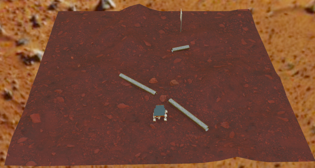
We conclude with a larger example of a Scenic program which also illustrates the language’s utility across domains and simulators. Specifically, we consider the problem of testing a motion planning algorithm for a Mars rover able to climb over hills and rocks. Such robots can have very complex dynamics, with the feasibility of a motion plan depending on exact details of the robot’s hardware and the geometry of the terrain. We can use Scenic to write a scenario generating challenging cases for a planner to solve in simulation. Some of the specifiers and operators we’ll use have not been discussed before in the tutorial; as usual, information about them can be found in the Syntax Guide.

We will write a scenario representing a hilly field of rocks and pipes with a bottleneck between the rover and its goal that forces the path planner to consider climbing over a rock. First, we import a small Scenic library for the Webots robotics simulator and a mars specific library which defines the (empty) workspace and several types of objects: the Rover itself, the Goal (represented by a flag), the MarsGround and MarsHill classes which are used to create the hilly terrain, and debris classes Rock, BigRock, and Pipe. Rock and BigRock have fixed sizes, and the rover can climb over them; Pipe cannot be climbed over, and can represent a pipe of arbitrary length, controlled by the length property (which corresponds to Scenic’s Y axis).

model scenic.simulators.webots.mars.model
from mars_lib import *

Here we’ve used the model statement to select the world model for the scenario: it is equivalent to from scenic.simulators.webots.model import * except that the choice of model can be overridden from the command line when compiling the scenario (using the --model option). This is useful for scenarios that use one of Scenic’s Abstract Domains: the scenario can be written once in a simulator-agnostic manner, then used with different simulators by selecting the appropriate simulator-specific world model.

Now we can start to create objects. The first object we will create will be the hilly ground. To do this, we use the MarsGround which has a terrain property which should be set to a collection of MarsHill classes, each of which adds a gaussian hill to the ground. Note that the MarsGround object has allowCollisions set to True, allowing objects to intersect and be slightly embedded in the ground. In the following code we create a ground object with 60 small hills (which are allowed to stack on top of each other):

ground = new MarsGround on (0,0,0), with terrain [new MarsHill for _ in range(60)]

We next create the rover at a fixed position and the goal at a random position on the other side of the workspace, ensuring both are on the ground:

ego = new Rover at (0, -3), on ground, with controller 'sojourner'
goal = new Goal at (Range(-2, 2), Range(2, 3)), on ground, facing (0,0,0)

Next we pick a position for the bottleneck, requiring it to lie roughly on the way from the robot to its goal, and place a rock there. Here we use the simple form of facing which takes a scalar argument, effectively setting the yaw of the object in the global coordinate system (so that 0 deg is due North, for example, and 90 deg is due West).

bottleneck = new OrientedPoint at ego offset by Range(-1.5, 1.5) @ Range(0.5, 1.5), facing Range(-30, 30) deg
require abs((angle to goal) - (angle to bottleneck)) <= 10 deg
new BigRock at bottleneck, on ground

Note how we define bottleneck as an OrientedPoint, with a range of possible orientations: this is to set up a local coordinate system for positioning the pipes making up the bottleneck. Specifically, we position two pipes of varying lengths on either side of the bottleneck, projected onto the ground, with their ends far enough apart for the robot to be able to pass between. Note that we explicitly specify parentOrientation to be the global coordinate system, which prevents the pipes from lying tangent to the ground as we want them flat and partially embedded in the ground.

gap = 1.2 * ego.width
halfGap = gap / 2

leftEdge = new OrientedPoint left of bottleneck by halfGap,
    facing Range(60, 120) deg relative to bottleneck.heading
rightEdge = new OrientedPoint right of bottleneck by halfGap,
    facing Range(-120, -60) deg relative to bottleneck.heading

new Pipe ahead of leftEdge, with length Range(1, 2), on ground, facing leftEdge, with parentOrientation 0
new Pipe ahead of rightEdge, with length Range(1, 2), on ground, facing rightEdge, with parentOrientation 0

Finally, to make the scenario slightly more interesting, we add several additional obstacles, positioned either on the far side of the bottleneck or anywhere at random (recalling that Scenic automatically ensures that no objects will overlap).

new Pipe on ground, with parentOrientation 0
new BigRock beyond bottleneck by Range(0.25, 0.75) @ Range(0.75, 1), on ground
new BigRock beyond bottleneck by Range(-0.75, -0.25) @ Range(0.75, 1), on ground
new Rock on ground
new Rock on ground
new Rock on ground

This completes the scenario, which can also be found in the Scenic repository under examples/webots/mars/narrowGoal.scenic. Scenes generated from the scenario, and visualized in Scenic’s internal visualizer and Webots, are shown below.

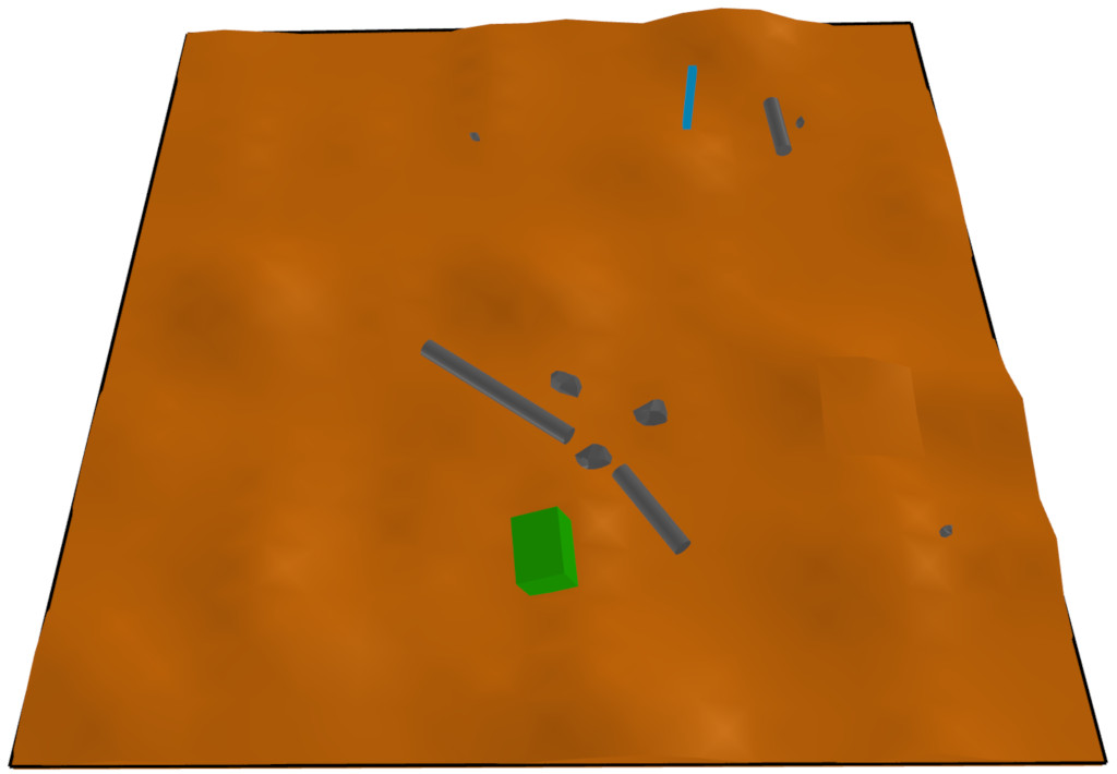
A scene sampled from the Mars rover scenario, rendered in Scenic’s internal visualizer.

A scene sampled from the Mars rover scenario, rendered in Webots.

Further Reading

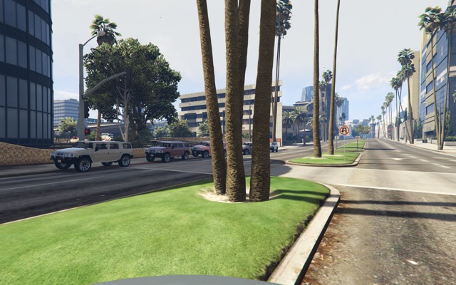
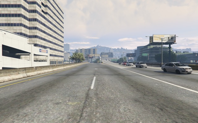
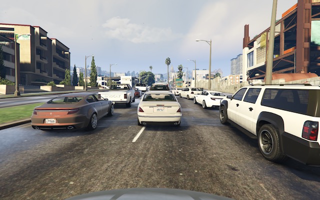
This tutorial illustrated the syntax of Scenic through several simple examples. Much more complex scenarios are possible, such as the platoon and bumper-to-bumper traffic GTA V scenarios shown below. For many further examples using a variety of simulators, see the examples folder, as well as the links in the Supported Simulators page.

Our tutorial on Dynamic Scenarios describes how to define scenarios with dynamic agents that move or take other actions over time. We also have a tutorial on Composing Scenarios: defining scenarios in a modular, reusable way and combining them to build up more complex scenarios.

For a comprehensive overview of Scenic’s syntax, including details on all specifiers, operators, distributions, statements, and built-in classes, see the Language Reference. Our Syntax Guide summarizes all of these language constructs in convenient tables with links to the detailed documentation.

Footnotes

[1]

Although collisions can be allowed on a per-object basis: see the allowCollisions property of Object.

[2]

Represented as an instance of the Orientation class, which internally uses quaternions (although you shouldn’t need to worry about that). In the rare case where you need to manipulate orientations beyond what Scenic’s operators provide, see the documentation for Orientation.

[3]

In fact, since ego is a variable and can be reassigned, we can set ego to one object, build a part of the scene around it, then reassign ego and build another part of the scene.

[4]

On the other hand, Scenic may have to work hard to satisfy difficult constraints. Ultimately Scenic falls back on rejection sampling, which in the worst case will run forever if the constraints are inconsistent (although we impose a limit on the number of iterations: see Scenario.generate).

References

[F22] (1,2)

Fremont et al., Scenic: A Language for Scenario Specification and Data Generation, Machine Learning, 2022. [Online]

[F19] (1,2,3)

Fremont et al., Scenic: A Language for Scenario Specification and Scene Generation, PLDI 2019.